Introduction
In this blog post, I’ll provide data stream background, applied context, motivation, and an overview for my recent work, Sketchy, co-authored with Xinyi Chen, Y. Jennifer Sun, Rohan Anil, and Elad Hazan, which will be featured in NeurIPS 2023 proceedings.
I really enjoyed working on this project because it simultaneously scratches different methodological itches of mine, from data stream sketching to online convex optimization. However, the algorithm introduced here was borne out of necessity; I didn’t go around with those two hammers a priori (though, presented with a nail, it made sense to reach for what’s readily available in my tool belt)!
This work is a big step in making matrix preconditioning training methods more accessible for deep learning by removing a critical memory bottleneck. For a deeper analysis, skip to the Motivation section below. Using matrix preconditioning training is probably one of the most under-appreciated techniques in modern neural network training, but for good reason. Shipping matrix preconditioning is quite challenging:
- It takes engineering work to eliminate overheads and numerical linear algebra bugs from the required matrix operations.
- Like any drastic optimizer change, it requires hyperparameter tuning.
- Like any drastic change, it requires socialization and “emotional work” to gain adoption, since everyone’s naturally risk-averse, especially to optimizer changes, since they are easy papers to write and thus its literature has a lot of noise.
- Organizational decision making is complex. An increase in quality demanding increased training compute will not sell, even if the exchange is favorable when converted to dollars. By trading off other factors, such as model or dataset size, a quality win can be converted to something Pareto dominant on all target teams’ desiderata.
I was quite lucky in that I didn’t need to start on these 4 challenges on my own! My mentor and manager, Rohan Anil did a lot of the initial labor here in shipping a version of the Shampoo optimizer. Sketchy breaks down a subsequent barrier to adoption for Shampoo, the memory usage.
Context
Here, I’ll discuss the research and production background that sets up for Sketchy. As the ML behind Google’s predicted click-thru-rate (pCTR) evolved, so too did its optimizer, often translating to quality wins. Better pCTR means more relevant ads selection means more money. Some public papers from Google provide great openly-available background.
The original 2013 View from the Trenches paper (which I’ve analyzed before on this blog) introduces a variant of AdaGrad called FTRL-Prox.
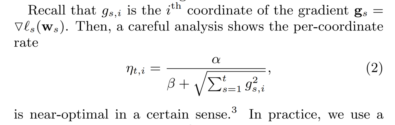
Rather than updating network weights with SGD given a gradient \(\textbf{g}_t\) using a fixed learning rate \(\textbf{x}_{t+1} = \textbf{x}_{t}-\eta\textbf{g}_t\), using the per-coordinate learning rates defined as above with updates \(x_{t+1, i} = x_{t, i}-\eta_{t,i}g_{t, i}\) (glossing over the lasso component here) dramatically improves optimization quality, due to a preconditioning effect. You can imagine how rescaling the \(x\) and \(y\) axes in the below level-plot of a 2D loss surface can result in faster optimization.
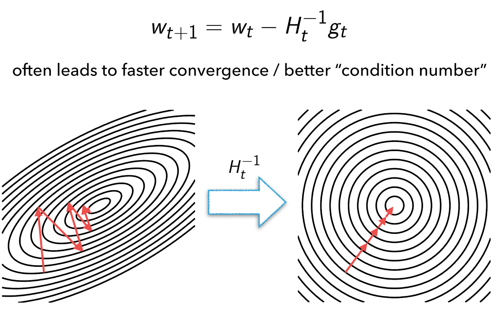
The magic of the AdaGrad’s analysis is in identifying that the running root-mean-square of the coordinate-wise gradients is the best such rescaling choice we can make in hindsight, up to a constant factor. Notice though, in the plot above, that the ellipses representing the parabolic loss surface on the left are rotated off-kilter: no rescaling of individual axes can transform the image on the left into the one on the right!
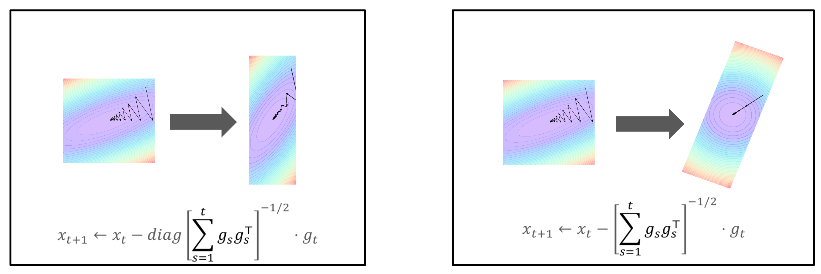
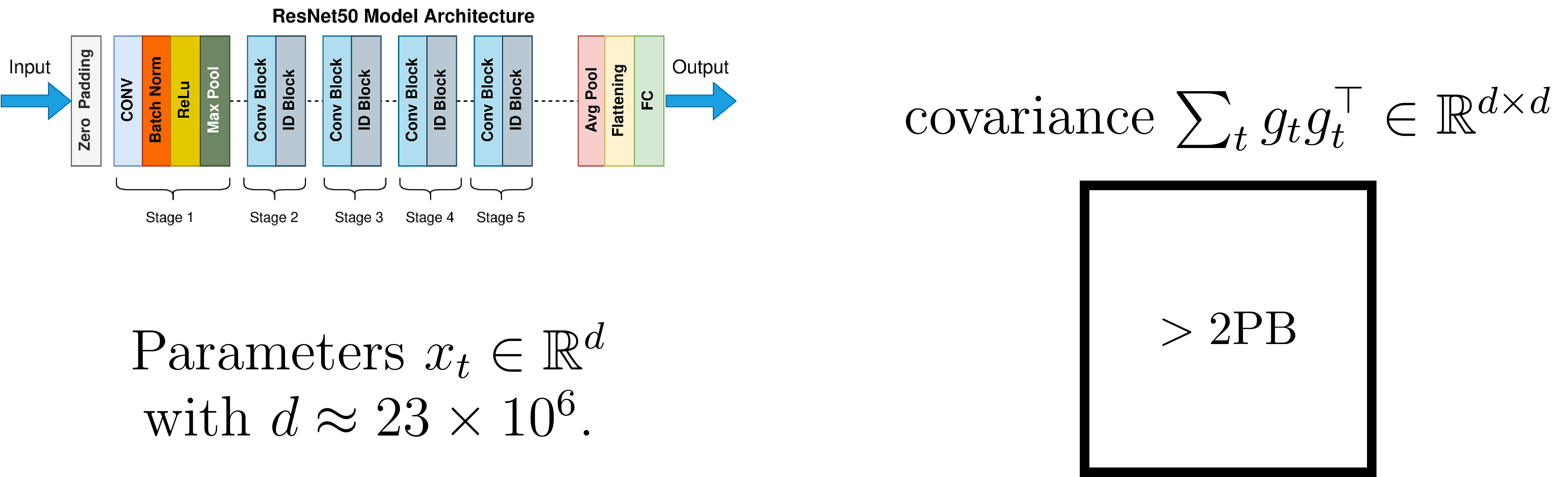
The problem here is that our gradients would be correlated across dimensions, and decorrelating them requires a full whitening matrix \(H_t^{-1}\) as pictured above. Unfortunately, this is a showstopper for all but the smallest problems. Full matrix Adagrad analysis states that the optimal preconditioner is the inverse matrix square root of the gradient covariance, \(C_t=\sum_t g_tg_t^\top\), the sum of gradient outer products. This would require petabytes to represent in modern neural networks!
Enter Shampoo. Shampoo tells us that for convex functions with matrix-shaped inputs, we can use a structured approximation to the full covariance \(C_t\) instead (DNNs are non-convex functions of multiple matrix-shaped inputs, but the convex-inspired approach seems to work!). In particular, given a weight matrix of shape \(a\times b\), rather than using the full flat gradient \(\textbf{g}_t\in\mathbb{R}^{ab}\), whose outer product is a matrix of size \(ab\times ab\), we can use the Kronecker product of reshaped matrix gradient’s tensor products. Specifically, we set
\[ G_t=\mathrm{reshape}\left(\textbf{g}_t, \left(a, b\right)\right)\,\,,\]
and then define the accumulated tensor products for both the left and right sides of the matrix gradient,
\[ L_t=\sum_{s=1}^tG_tG_t^\top\,\,\,\,;\,\,\,\,R_t=\sum_{s=1}^tG_t^\top G_t\,\,,\]
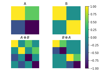
where \(L_t,R_t\) are of shape \(a\times a,b\times b\), respectively. Then the Kronecker product \(L_t\otimes R_t\approx C_t^2\), in the sense that we can recover regret guarantees similar to full matrix AdaGrad when using the former. The Kronecker product thus can be viewed as an approximation of the \(C_t\) matrix of \((ab)^2\) entries using \(a^2+b^2\) entries instead. I’ve gone into detail on the Kronecker product from a computation perspective in a walkthrough notebook, but as a little demo, see below.
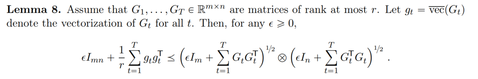
The critical part of the Shampoo paper which relates the approximation to \(C_t\) is in Lemma 8, which I excerpt below but won’t go into detail on.
So, are we done? Not quite. For the ever-ubiquitous Transformers, highly rectangular weights are common, e.g., take the big transformer, which has \(a=1024\) and \(b=4a\) (these are models from 2017; nowadays we have bigger ones but \(b/a\) tends to be at least 4). Shampoo’s memory overhead here would be around \(2(1 + 16)a^2\), since you need to store the statistics \(L_t,R_t\) and their matrix inverse roots. Remember, the full parameter has size \(4a^2\)!
Nowadays, when you’re getting ready to train a transformer, or whatever, you don’t set aside enough room in your GPU memory for 8 more copies of the model, you train a bigger model.
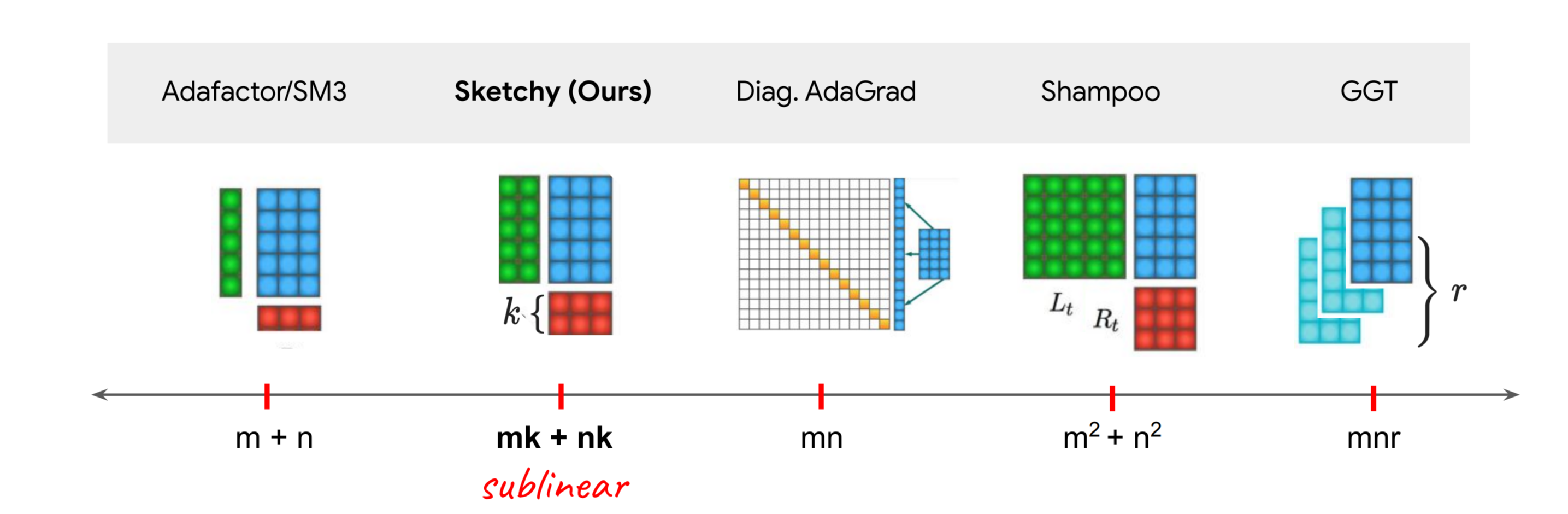
This is where Sketchy enters the picture: can we retain the quality wins of Shampoo but drop memory to AdaGrad/Adam levels? Previous work like AdaFactor shows we can give up quality to reduce memory. But can we leverage second moment information to use less memory than Adam and still beat it?
Motivation
Besides wanting to have Shampoo quality without its memory prices, there are deep trends in computing which suggest memory reduction is worth investing in.
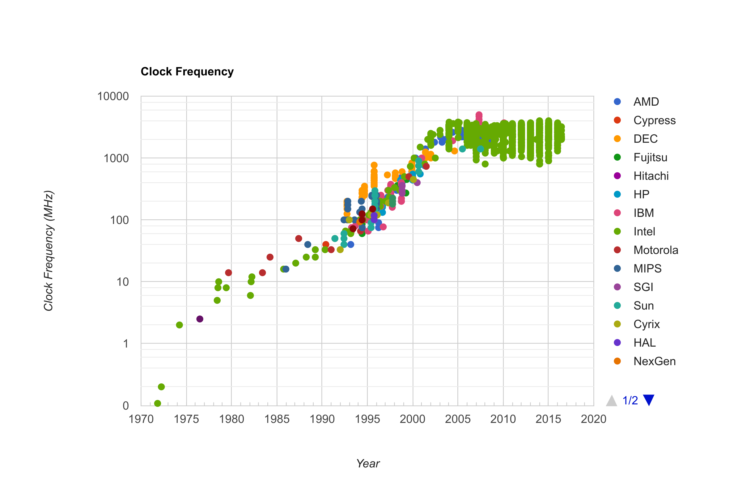
Batch size. We’ve all seen the clock speed charts and parallelism is the future arguments already; hardware acceleration via parallelism has won. Here’s an indicative plot from CPUDB:
OK, so say in the future you buy that training will have more parallel devices each contributing FLOPS rather than more FLOPS per device. What does that tell us about optimizers? That we can afford to do fancier operations in our optimizers, which usually (and with ZeRO especially) are not a meaningful amount of compute compared to the rest of DNN training!
If you have many devices, and therefore large batch sizes, training your neural network, then any optimizer which only processes the mini-batch gradient (e.g., not K-FAC) effectively has its step time amortized per example in the batch. Note that this falls out of the fact that your gradient shape is independent of the batch size. If you can spend the time to make a higher-quality step from each gradient, then do so!
Memory Bandwidth. Device logic is speeding up faster than memory access speed. There are fundamental reasons we should expect algorithms with high compute density (compute per memory access) to be faster. But more practically speaking, there’s growing headroom in physical devices where we should be looking to find better ways of optimizing our network by increasing compute per memory access (e.g., from loading of an example or weights).
| Device Family | Compute Increase | Memory Bandwidth Increase | ||||||||
|---|---|---|---|---|---|---|---|---|---|---|
| TPUv2 to TPUv3 | 2.67× | 1.29× | ||||||||
| V100 to A100 | 5× | 2.2× |
This means that if we have an algorithm that improves quality while using nearly the same amount of memory bandwidth (e.g., it is a low-memory optimizer which is applied to the same-size neural net and requires scanning through the same number of examples), but perhaps more compute, then we expect this algorithm to speed up over time as compute increases faster than memory bandwidth.
Overview
On the face of it, we should be suspect that we can use asymptotically equivalent memory to Adam and still achieve near-Shampoo levels of quality (there are other buffers which require memory linear in parameter size, for learning rate grafting, momentum, etc.).
So we should clarify how we can take advantage of problem-specific structure to reduce memory use.
The key is that \(L_t,R_t\) (or moving average analogues of the two, in the non-convex NN case) exhibit fast spectral decay. In other words, a low rank plus diagonal approximation to each of those two matrices suffices to preserve the matrix action of each one individually.
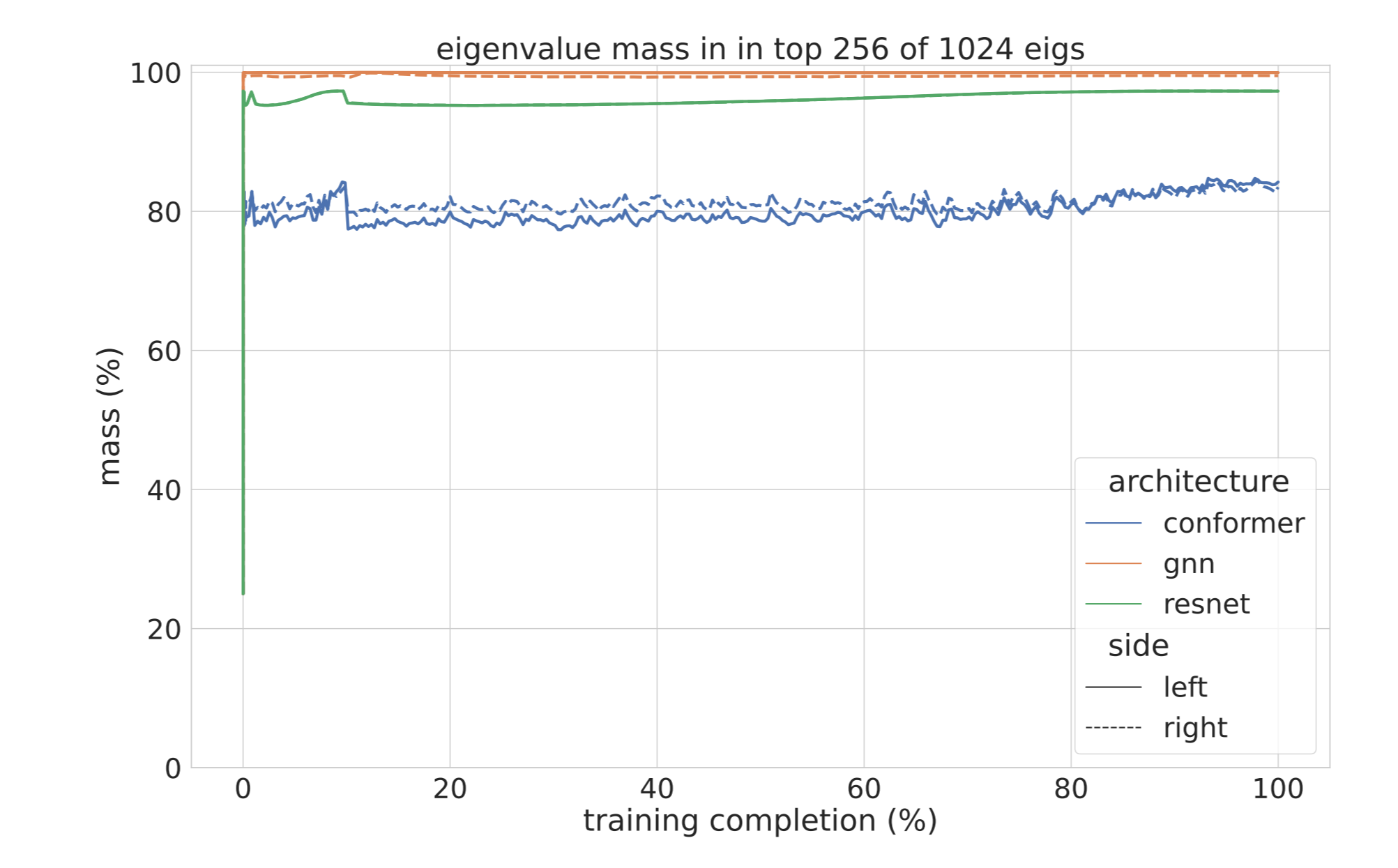
The plot above shows that taking the top 25% of the eigenvalues for a weight with an axis of size 1024 is enough to capture over 80% of the spectral mass in those statistics, across architectures, throughout training.
This is a highly nontrivial property—note that in fact we have a rotating top-subspace over the course of training for the EMA version \(L_t=\sum_{s\le t}\beta^{t-s}G_sG_s^\top\). If we just had a \(256\times 1024\) weight matrix with normal gradients, we’d see a near isometry when EMA’ing:
import numpy as np
from jax.config import config
config.update("jax_enable_x64", True)
from jax import numpy as jnp
rng = np.random.default_rng(1234)
d, n, beta = 256, 10000, 0.999
x = rng.normal(size=(n, 1024, d))
# reverse sort for numerical stability, note square root b/c we square x.
x *= np.power(beta, np.arange(n) / 2)[::-1, np.newaxis, np.newaxis]
cov = 0
for i in range(0, 10000, 1000):
  s = x[i:i + 1000]
  cov += jnp.einsum('nxd,nyd->xy', s, s).block_until_ready()
eigvals = np.linalg.eigvalsh(cov)
eigvals[-256:].sum() / eigvals.sum()  # 26.5%
But simply knowing a low rank approximation would do isn’t enough. You’d need the SVD (or iterative top-\(k\) variants of it) applied to the full statistics to compute this low rank approximation. But if we’re tracking full statistics, we’re already paying for \(a^2+b^2\) space!
Can we approximate the low rank approximation of a matrix, here, \(C_t=\sum_{s\le t}G_sG_s^\top\), using only the space of the low rank approximation itself incrementally updating our approximation, having each \(G_s\) revealed to you?
This seems impossible at first sight (indeed, the exact problem is). How can you both track the current top eigenspace and also update it as you go along? It’d be like trying to find the top-\(k\) most frequent unique items in a data stream using only \(O(k)\) memory, except the eigenvalue version of that.
This happens to be exactly the observation Edo Liberty made when introducing Frequent Directions (FD). Indeed, as my co-author Elad Hazan pointed out, if you trace the FD algorithm with incoming vectors equal to basis vectors, you recover Misra-Gries (the algorithm solving the frequent item stream challenge in the previous paragraph).
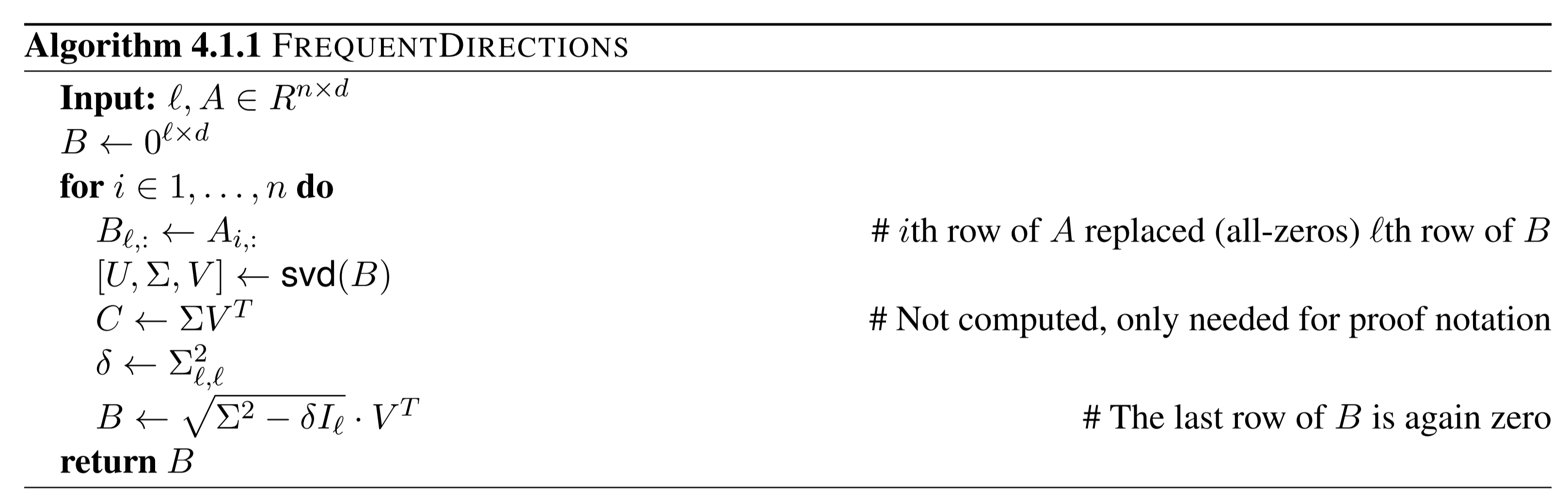
In the above, the sketch \(B_i\) has the property that \(B_i^\top B_i\) approximates the covariance \(A_i^\top A_i\) in operator norm, with error that scales in the lowest \(d-\ell\) singular values of \(A_i\).
Replace \(A_i\) with \(C_t\) and we have the opportunity to apply sketching for second moment capture! The real work in Sketchy came in not from the idea of applying sketches to data streams, but from proving that the approximation from FD can be made good-enough to use for optimization, and that your error at the end of optimizing also only depens on lower-order eigenvalues of your gradient covariance.
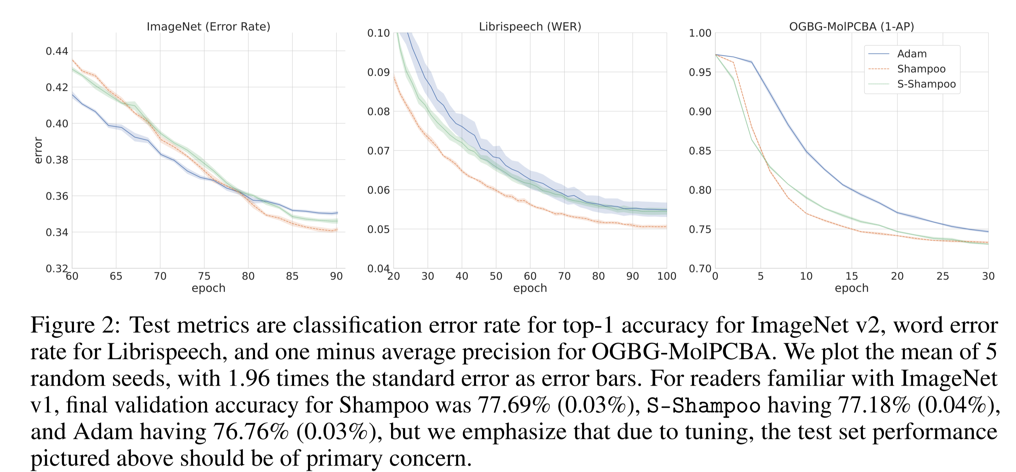
We were heartened by the test performance of the optimizer against Adam and Shampoo, landing in between the linear and super-linear optimizers in terms of quality.
This overview post barely touched on the algorithms involved in Sketchy, and only alluded to the theoretical details, all of which can be found in the full paper. There’s also a completely separate half to this paper which we didn’t have space to get into: the computational aspect of it! We used full SVD for the theoretical paper results, but it’s possible to exploit iterative top-singular-value routines instead.
We’re eager to work on these solutions with you! Reference Jax code is available on github, and please reach out if you’re interested in a pytorch or iterative top-k eigenvalue implementation!