Distillation Walkthrough
Distillation is a critical technique towards improving a network’s quality while keeping its serving latency constant.
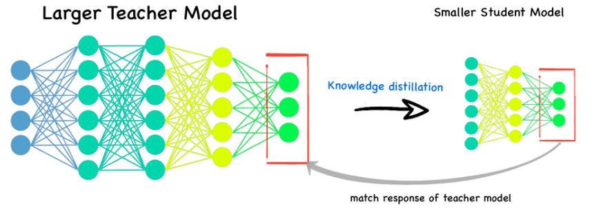
This is becoming crucial as people focus on serving larger and larger models. Image found on LinkedIn.
Distillation is a powerful technique, but a couple things about it are quite mystical. The purpose of this post is to:
- Provide a very high level explainer (but mostly refer to source papers) of distillation.
- Show that you can create a simple, linear example where distillation works.
How is distillation implemented?
At an algorithmic level, distillation, introduced by Hinton, Vinyals, and Dean 2015, applied to a classification problem with labels \(y=1,\cdots,d \) proceeds as follows.
- Train a large, expensive teacher network \(T(x;\mu) \) to predict the distribution \(y|x \) (a categorical distribution on \([d] \), \(\Delta_d \)) from a large dataset of \((x, y) \) pairs; this is done by minimizing negative log-likelihood (NLL) of the teacher’s prediction \(\min_\mu -\log T(x; \mu)_y \), yielding \(\mu_* \).
- Train your smaller, cheaper network \(S(x;\theta) \) on a combined loss from the data NLL and matching the teacher distribution by minimizing cross-entropy \(H(T(x;\mu_*),S(x;\theta))=-\sum_{i=1}^d T(x; \mu_*)_i\log S(x; \theta)_i\), i.e., \(\min_\theta -\log S(x; \theta)_y + \alpha H(T(x;\mu_*),S(x;\theta)) \). Since \(\mu_* \) is fixed, optimizing the latter term is equivalent to minimizing \(D_{\mathrm{KL}}(T||S) \), where \(\alpha \) is some hyper.
This has been scaled up to language models too, see Anil et al 2018.
Why wouldn’t it work?
At first, I found the fact that distillation helps mind-bending. To understand why I was confused, let’s look at the distillation loss for \(\theta \):
\[ -\log S(x; \theta)_y + \alpha H(T(x;\mu_*), S(x;\theta)) = c_\alpha H\left(\frac{\delta_y +\alpha T(x;\mu_*)}{1+\alpha},S(x;\theta)\right) \]
That is, distillation loss is, up to a constant \(c_\alpha \), equivalent to softening our data label \(y \) by the teacher’s predictions \(T(x;\mu_*) \). Above, $\delta_y$ stands for the atomic distribution which concentrates all the mass on \(y\); we perform a weighted average with the teacher distribution for the label \(T(x;\mu_*)\).
We started with a dataset. Ran it through some matmuls, \(T(x;\mu_*) \). So if we view the dataset as a huge random variable (rv) \(D \), \(\mu_* \) and indeed \(T(x;\mu_*) \) is just some other rv which is a very complicated function of \(D \) (since they resulted from SGD or some training process applied to \(D \)).
So we just took our clean labels \(y \) and added noise to them! And it helped! Indeed, we can formalize this concern in the case \(\alpha=\infty \) (so that the distillation label \(y’=T(x;\mu_*) \)). In practice, and even in the linear setting I discuss next, this still works, in that train and test loss improve over using \(y \).
If we train with just \(y’ \) then the training process forms a Markov chain conditioned on all \(x \): \(y \rightarrow \mu_*\rightarrow \theta_* \) (given \(\mu_* \), and therefore \(y’ \), the training of \(\theta_* \) is conditionally independent of \(y \)).
Then by the data processing inequality, the mutual information \(I(y, \mu_*)\ge I_{\alpha=\infty}(y, \theta_*) \).
This implies that, in the case of self-distillation, where you can globally optimize the learner (find the true minimum \(\mu_*,\theta_*\)), we shouldn’t expect any improvement over the teacher—this would violate the DPI!
There’s no paradox with the example below, since our teacher is of a different class than the student, but, still, it feels wrong to distance ourselves from the true label. We don’t know the relationship between \( I_{\alpha=\infty}(y, \theta_*) \) and \( I_{\alpha=0}(y, \theta_*) \) but this seems like a step in the wrong direction.
This concern could be framed as an invocation Vapnik’s principle: “When solving a problem of interest, do not solve a more general problem as an intermediate step.”
Why does it work?
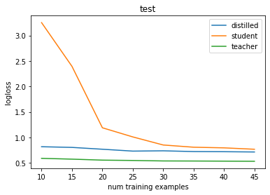
In short, it can be the case that \( I_{\alpha=\infty}(y, \theta_*) > I_{\alpha=0}(y, \theta_*) \) because of variance reduction for a finite dataset (showing equality in the data limit would be quite interesting, reach out to me if you have that result!). The teacher makes the labels less noisy.
The underlying classification problem has \((X, Y)\sim\mathcal{D} \) where noisy \(Y|X \) is still stochastic. One can imagine that for a logistic loss, the variance of the training loss from \(n \) examples derived from the dataset \((X, \mathbb{E}[Y|X]) \) is smaller than that of the training loss from \(n \) examples of \((X, Y) \). For a probabilistic binary model \(p_\theta \) parameterized by \(\theta \):
\[ \mathrm{var}\ \frac{1}{n}\sum_i\log(1+\exp(-Y_ip_\theta(X_i)))\ge \mathrm{var}\ \frac{1}{n}\sum_i\log(1+\exp(-\mathbb{E}[Y_i|X_i]p_\theta(x_i)))\,\,, \]
where this holds by Jensen and the fact that log loss is convex (note this still holds for neural nets \(p_\theta \)).
So if instead of \(\mathbb{E}[Y|X] \) we use a larger neural network teacher \(\hat f(X)\approx \mathbb{E}[Y|X] \), so long as the teacher itself does not add more variance to our training objective, then knowledge distillation can indeed be useful.
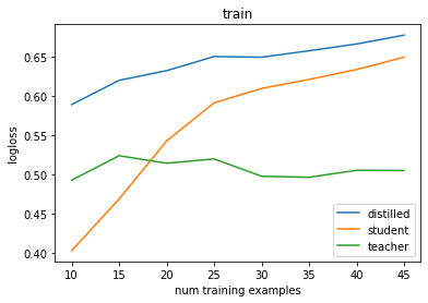
The below shows a non-deep simple example in the low-data setting where this matters, but again, we rely on the fact that the teacher has a strong inductive bias so that the last caveat is met.
import numpy as np
from sklearn.base import clone
from sklearn.preprocessing import PolynomialFeatures, FunctionTransformer
from sklearn.pipeline import make_pipeline
from sklearn.linear_model import LogisticRegression, LinearRegression
from sklearn.model_selection import train_test_split
from scipy.special import expit
from sklearn.metrics import log_loss
def base_distribution(rng, n):
  x = rng.standard_normal(n) * 10
  ey = 0.4 * np.sin(x) + 0.5
  y = rng.binomial(1, ey)
  return x[:, np.newaxis], y
def run_kd(num_training_ex, x, y):
  test_prop = 1 - num_training_ex / len(x)
  xtr, xte, ytr, yte = train_test_split(x, y, test_size=test_prop, random_state=42)

  # Student is from a model class that won't be able to reconstruct the ground
  # truth
  degree = 3
  student = make_pipeline(
      PolynomialFeatures(degree),
      LogisticRegression(max_iter=1000))

  # Teacher comes from a better model class
  teacher = make_pipeline(
      FunctionTransformer(np.sin),
      LogisticRegression(max_iter=1000))

  student.fit(xtr, ytr)
  teacher.fit(xtr, ytr)

  teacher_labels = teacher.decision_function(xtr)

  # Hack to train on soft targets
  # https://stackoverflow.com/a/60969923

  distilled = make_pipeline(
      PolynomialFeatures(degree),
      LinearRegression())

  distilled.fit(xtr, teacher_labels)
  distilled.decision_function = distilled.predict

  models = {'student': student, 'teacher': teacher, 'distilled': distilled}
  datasets = {'train': (xtr, ytr), 'test': (xte, yte)}

  results = {}

  for model_name, model in models.items():
    for split_name, (x, y) in datasets.items():
      pred = model.decision_function(x)
      pred = expit(pred)
      results[model_name + '.' + split_name] = log_loss(y, pred)

  return results
results = None
ntrials = 15
import jax
nexs = np.arange(10, 50, 5, int)
for nex in nexs:
  rng = np.random.default_rng(1234)
  trials = [run_kd(nex, *base_distribution(rng, 10000)) for _ in range(ntrials)]
  # List of dicts to dict of singleton list of average
  run = jax.tree_map(lambda *xs: [np.mean(xs)], *trials)
  results = run if not results else {k: results[k] + run[k] for k in results}
from matplotlib import pyplot as plt

for split in ['train', 'test']:
  for k, v in results.items():
    if split in k:
      plt.plot(nexs, v, label=k.replace('.' + split, ''))
  plt.legend()
  plt.title(split)
  plt.xlabel('num training examples')
  plt.ylabel('logloss')
  plt.show()
Is that all there is to it?
Not quite. With neural nets, we do see some really interesting training phenomena not fully accounted for by the story above. For instance, self-distillation (where the “teacher” is the same size as the student) somehow works!
There are interactions with imperfect non-convex optimization in the deep neural network setting which are still a research topic. For more, check out a Zeyuan Allen-Zhu and Yuanzhi Li blog post from MSR.