Numpy Gems 1: Approximate Dictionary Encoding and Fast Python Mapping
Welcome to the first installment of Numpy Gems, a deep dive into a library that probably shaped python itself into the language it is today, numpy.
I’ve spoken extensively on numpy (HN discussion), but I think the library is full of delightful little gems that enable perfect instances of API-context fit, the situation where interfaces and algorithmic problem contexts fall in line oh-so-nicely and the resulting code is clean, expressive, and efficient.
What is dictionary encoding?
A dictionary encoding is an efficient way of representing data with lots of repeated values. For instance, at the MovieLens dataset, which contains a list of ratings for a variety of movies.
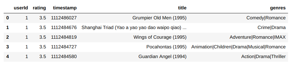
But the dataset only has around 27K distinct movies for over 20M ratings. If the average movie is rated around 700 times, then it doesn’t make much sense to represent the list of movies for each rating as an array of strings. There’s a lot of needless copies. If we’re trying to build a recommendation engine, then a key part of training is going to involve iterating over these ratings. With so much extra data being transferred between RAM and cache, we’re just asking for our bandwidth to be saturated. Not to mention the gross overuse of RAM in the first place.
That’s why this dataset actually comes with movieIds, and then each rating refers to a movie though its identifier. Then we store a “dictionary” mapping movie identifiers to movie names and their genre metadata. This solves all our problems: no more duplication, no more indirection, much less memory use.
That’s basically it. It’s a very simple encoding, which makes it easy to integrate efficiently in many algorithms. So much so, that many, many libraries natively support dictionary encoding your data–see factors in R and pandas.
Why approximate?
Let’s run with our example. Suppose we have a list of our movie titles, and we’re doing some NLP on them for better recommendations. Usually, that means each of these movies correspond to some kind of encodings.
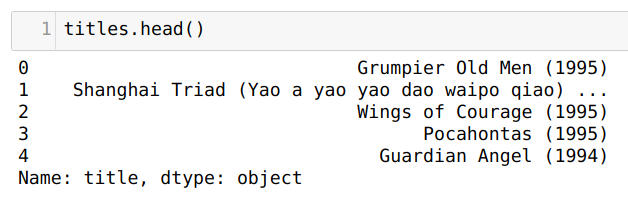
Let’s use the built-in pandas categorical dtype, which is a dictionary encoding.
len(titles) # ---> 20000263
cat_titles = titles.astype(
    pd.api.types.CategoricalDtype(
        pd.unique(titles)))
len(cat_titles.cat.categories) # ---> 9260
len(cat_titles.cat.codes) # ---> 20000263
This stores our data into a densely packed array of integers, the codes, which index into the categories array, which is now a much smaller array of 9K deduplicated strings. But still, if our movie titles correspond to giant floating-point encodings, we’ll still end up shuffling a bunch of memory around. Maybe 9K doesn’t sound so bad to you, but what if we had a larger dataset? Bear with this smaller one for demonstration purposes.
A key observation is that, like most datasets, we’ll observe a power-law like distribution of popularity:
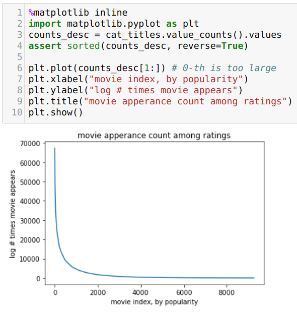
What this means is that we have a long tail of obscure movies that we just don’t care about. In fact, if we’re OK dropping 5% coverage, which won’t affect our performance too much, we can save a bunch of space.
cdf = counts_desc.cumsum() / counts_desc.sum()
np.searchsorted(cdf, [.95, .99, .999, 1])
# ---> array([3204, 5575, 7918, 9259])
Indeed, it looks like dropping the 5% least-popular movies corresponds to needing to support only 1/3 as many movies overall! This can be a huge win, especially if your model considers higher-order interactions (if you like movie X and movie Y, then you might like movie Z). In such models that 1/3 becomes a 1/27th!
How to approximate?
However, if we’re being asked to serve model predictions online or want to train a “catch-all” encoding, then we still need to have a general catch-all “movie title” corresponding to the unknown situation. We have a bunch of dictionary indices in [0, d), like [1, 3, 5, 2, 6, 1, 0, 11]. In total we have n of these. We also have a list of e items we actually care about in our approximate dictionary, say [5, 8, 10, 11], but this might not be a contiguous range.
What we want is an approximate dictionary encoding with a catch-all, namely we want to get a list of n numbers between 0 and e, with e being the catch all.
In the above example, n = 8, d = 12, e = 4, and the correct result array is [4, 4, 0, 4, 4, 4, 4, 3]. For something like embeddings, it’s clear how this is useful in greatly reducing the number of things we need to represent.
The Gem
The above is actually an instance of a translation problem, in the sense that we have some translation mapping from [0, d) into [0, e] and we’d like to apply it to every item in the array. Like many things in python, this is most efficient when pushed to C. Indeed, for strings, there’s translate that does this.
We’ll consider two dummy distributions, which will either be extremely sparse (d > n) or more typical (d <= n). Both kinds show up in real life.
We extract the most popular e of these items (or maybe we have some other metric, not necessarily popularity, that extracts these items of interest).
There are more efficient ways of doing the below, but we’re just setting up.
if d < n:
    dindices = np.random.geometric(p=0.01, size=(n - d)) - 1
    dindices = np.concatenate([dindices, np.arange(d)])
    dcounts = np.bincount(dindices)
    selected = dcounts.argsort()[::-1][:e]
else:
    dindices = np.random.choice(d, n // 2)
    frequent = np.random.choice(n, n - n // 2)
    dindices = np.concatenate([dindices, frequent])
    c = Counter(dindices)
    selected = np.asarray(sorted(c, key=c.get, reverse=True)[:e])
Let’s look at the obvious implementation. We’d like to map contiguous integers, so let’s implement a mapping as an array, where the array value at an index is the mapping’s value for that index as input. This is the implementation that pandas uses under the hood when you ask it to change its categorical values.
mapping = np.full(d, e)
mapping[selected] = np.arange(e)
result = np.take(mapping, dindices)
As can be seen from the code, we’re going to get burned when d is large, and we can’t take advantage of the fact that e is small. These benchmarks, performed with %%memit and %%timeit jupyter magics on fresh kernels each run, back this sentiment up.
e |
d |
n |
memory (MiB) | time (ms) |
|---|---|---|---|---|
10^3 |
10^4 |
10^8 |
763 | 345 |
10^3 |
10^6 |
10^6 |
11 | 9.62 |
10^3 |
10^8 |
10^4 |
763 | 210 |
10 |
10^4 |
10^8 |
763 | 330 |
10 |
10^6 |
10^6 |
11 | 9.66 |
10 |
10^8 |
10^4 |
763 | 210 |
This brings us to our first puzzle and numpy gem. How can we re-write this to take advantage of small e? The trick is to use a sparse representation of our mapping, namely just selected. We can look in this mapping very efficiently, thanks to np.searchsorted. Then with some extra tabulation (using -1 as a sentinel value), all we have to ask is where in selected a given index from dindices was found.
searched = np.searchsorted(selected, dindices)
selected2 = np.append(selected, [-1])
searched[selected2[searched] != dindices] = -1
searched[searched == -1] = e
result = searched
A couple interesting things happen up there: we switch our memory usage from linear in d to linear in n, and completely adapt our algorithm to being insensitive to a high number of unpopular values. Certainly, this performs horribly where d is small enough that the mapping above is the clear way to go, but the benchmarks expose an interesting tradeoff frontier:
| ` e ` | ` d ` | ` n ` | memory (MiB) | time (ms) |
|---|---|---|---|---|
10^3 |
10^4 |
10^8 |
1546 | 5070 |
10^3 |
10^6 |
10^6 |
13 | 31 |
10^3 |
10^8 |
10^4 |
0.24 | 0.295 |
10 |
10^4 |
10^8 |
1573 | 1940 |
10 |
10^6 |
10^6 |
13 | 17 |
10 |
10^8 |
10^4 |
0.20 | 0.117 |