Markov Chain Monte Carlo methods (MCMC) are, functionally, very cool: they enable us to convert a specification of a probability distribution from a likelihood \(\ell\) into samples from that likelihood. The main downside is that they’re very slow. That’s why lots of effort has been invested in data-parallel MCMC (e.g., EPMCMC). This blog post takes a look at a specialized MCMC sampler which is transition-parallel, for a simple distribution:
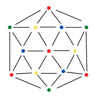
Given a fixed, simple, large graph \(G=(V,E)\) on \(n\) vertices and \(m\) edges, return a uniform proper random \(k\)-coloring, where \(k > 2\Delta(G)\) and \(\Delta=\Delta(G)\) is the maximum degree of \(G\)
Such a sampler could be used to generate colorings with generalization properties for machine learning or simulating Glauber dynamics in physical systems.
Note that while it’s easy to state this distribution as drawing a random element from the combinatorial structure \[ \left\{v\in[k]^n\, \big|\, v_i\neq v_j\,\,\forall (i,j)\in E\right\}\,, \] it’s far from trivial to actually do so (of course, we make colors synonymous with numbers here). Sure, every marginal distribution of every vertex is just uniform, but complex dependencies across vertices arise: highly central nodes can significantly affect permissible colors for other nodes.
For the given problem, Jerrum provides a classic Gibbs sampler:
- Perform any proper greedy coloring of \(G\).
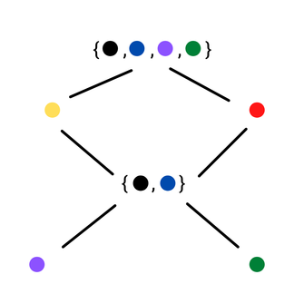
- Repeatedly, sample a vertex and resample its color uniformly from the set of colors among \([k]\) absent from its neighbors.
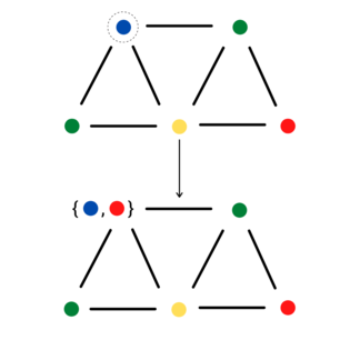
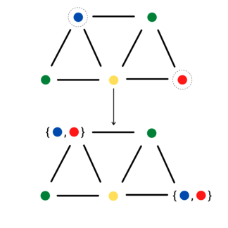
Note, the image above uses curly braces to denote the uniform random outcome of the above sampling step—for a given chain, only one color will be chosen.
This works fine and is considered fast-mixing, but is single-threaded. You have to loop on the “repeatedly” step for the Markov chain (MC) to burn in. Choosing the smallest legal \(k\), the mixing time is \(\tilde{O}(\Delta m)\).
We can make a simple observation here: our graph \(G\) describes the MRF for the interdependent random variables defining the color of each vertex in \(V\). That’s just a fancy way of saying: conditioned on your neighbor’s colors, your color is a uniform independent random variable over the remaining colors, ignorant of the color of any other vertex. In turn, suppose over the course of Jerrum’s algorithm we were to sample two vertices \(v, w\) at least distance 2 apart. As far as the MC is concerned, we might as well transition \(v\) and \(w\) in parallel!
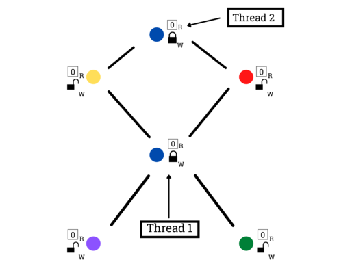
This leads us to a naively parallel sampler, attaching RW locks to each vertex.
- Perform any proper greedy coloring of \(G\)
- On many threads, repeatedly:
- Uniformly sample a vertex \(v\)
- Try to write-lock \(v\) (upon failure, restart at (2-1))
- Try to read-lock all neighbors of \(v\) (upon failure, restart at (2-1))
- Resample a color for \(v\) based on the read-locked snapshots
Pictorially, after sampling a vertex on each thread (2-1), threads continue to acquire write locks (2-2):
Then they grab neighbor read locks (2-3):
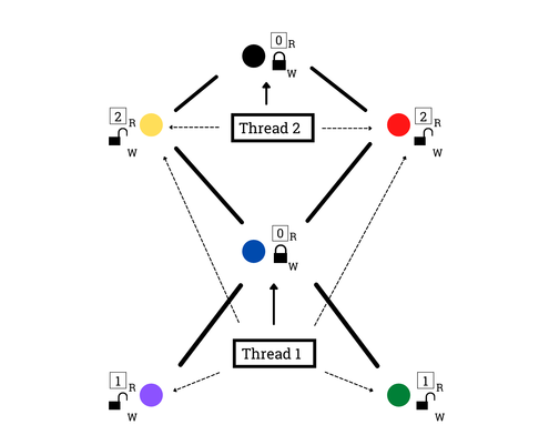
And finally, they perform resampling and unlock (2-4):
Now we have a natively transition-parallel sampler. The only catch is what happens when we fail to acquire a lock. If a thread just unlocks everything and tries to grab another vertex, then we’re no longer perfectly replicating Jerrum’s sampler: we’re going to implicitly favor updating the color of lower-degree vertices since they’ll have less conflicts.
There might be ways to counter this, e.g., non-uniform sampling in part (2-1), restarting at step (2-2) instead of step (2-1), etc., but an interesting question is “who cares?” because the increased sampling rate could mean we can get to some (possibly asymptotically biased) samples faster.
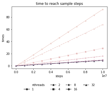
Here’s a plot of how long it takes to reach a given transition step count across various levels of parallelism using the sampler above (on a fixed, randomly sampled connected graph of 1M vertices and average degree 100). Time here is in seconds.
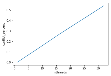
As we increase the number of threads, so too does the percentage of unsuccessful lock attempts, as expected. However, for this sparse graph, even with 32 threads (this is hyperthreading 2x for 16-core machine), the percentage of lock attempts that are unsuccessful remains less than about half a percent.
Despite using biased transition dynamics (but only slightly so, as the above demonstrates), natural parallelism within our MRF makes the “just use more cores” approach appealing for sparse graphs. This was all a ton of fun to code up, and had lots of little interesting systems problems:
- How would one actually build this many fast RW locks?
- How might one avoid deadlock?
- How can we leverage Rust’s type system to enforce lightweight atomics-based lock guards on our graph?
Check the repo out here.
There’s a lot further one could take this: I’m sure you’d want to partition \(G\) and only use locks at partition boundaries, for instance, as well as debias the parallel sampling process by changing how to sample \(v\). But the upshot to me is that MRFs provide a natural mechanism for interior parallelism when performing MCMC sampling.
Illustrations provided by Olivia Wynkoop.